Improving Pipeline Failure Prediction via Data Sanitization, Hyperparameter Optimization, and Boosting Blending Ensembles

Abstract

This paper addresses the task of predicting failure risks in municipal district heating (centralized hot water supply) and water distribution pipeline networks. We present a systematic, stage-by-stage methodology for improving the generalization capability of AI-based predictive models. We describe the transition from a baseline classifier trained on noisy data to a sanitized database, hyperparameter optimization, and the construction of a multi-model blending ensemble combining XGBoost, CatBoost, LightGBM, and classical Gradient Boosting algorithms. The implementation of the proposed pipeline increases the risk ranking metric ROC-AUC from a baseline of 0.7243 to 0.8879 for continuous risk score predictions, while boosting prediction accuracy in the highest risk zone (Precision@20) to 90.0%.

1. Introduction and Baseline Formulation (Stage 1)

Failure prediction on pipeline segments is a critical task for municipal utilities and energy companies. Timely identification of high-risk areas allows operators to optimize inspection budgets, plan preventive maintenance, and minimize consumer service interruptions.

In the initial stage of this study, we formulated a binary classification task to predict the probability of failure occurrences on pipeline segments (Sys) during the subsequent year. The target variable ( $Y$ ) represented the registration of at least one failure incident. The baseline model was trained on the raw, noisy dataset containing historical dispatch logs.

A single classifier based on the standard Gradient Boosting algorithm was deployed as the baseline. The evaluation on the independent test set (year 2023) yielded suboptimal classification performance:

ROC-AUC: 0.7243
Accuracy: 74.22%
Precision: 49.54%
Recall: 55.10%
F1-Score: 0.5217
Precision at Top-20 Risks (Precision@20): 80.00%

An analysis of the training process revealed severe convergence instability. The learning curves exhibited substantial high-frequency noise and sudden metric drops, indicating conflicting labels and data entry errors in the training dataset.

2. Data and Features

The predictive models are trained on an integrated database consisting of physical and technical pipeline characteristics and historical failure logs.

2.1. Spatial Structure: Sys and Section

The spatial network layout is represented at two levels of granularity:

Sys — an elementary pipeline segment (a continuous pipe segment of constant diameter between two junctions or chambers). This is the finest spatial unit in the database. The dataset contains 8,243 unique Sys segments.
Section — an aggregated network section (e.g., street-level pipeline, local distribution line, or main transmission conduit) combining several contiguous Sys segments. In practice, utility rehabilitation decisions are made at the Section level. The network comprises 1,920 unique Section units.

Failure probabilities are predicted at the micro-level (Sys) and subsequently aggregated to the macro-level (Section) using the maximum operator: $P (Section_{i}) = max_{j \in Sys (i)} P (Sys_{j})$

2.2. Failure History and Statistics

The study period spans from 2019 to 2025. The temporal distribution of failures aggregated at the section level is presented in Table 1.

Table 1. Distribution of the Target Class and Failure Incidents by Year

Year	Total Sections	Positive Sections (Failures)	Positive Rate (%)	Total Registered Events
2019	1920	223	11.61%	471.0
2020	1920	260	13.54%	593.0
2021	1920	278	14.47%	661.0
2022	1920	298	15.52%	892.0
2023	1920	331	17.24%	1133.0
2024	1920	340	17.71%	1243.0
2025	1920	378	19.69%	1591.0

The data shows a steady upward trend in registered incidents due to infrastructural aging, as well as a significant class imbalance (approximately 85% of sections remain failure-free each year).

2.3. Input Features

The feature vector for each sample consists of 107 variables, classified into three main groups:

Static Numerical Features (25 features): segment length, burial depth, nominal diameter, wall thickness, operating pressure, age (construction year), thermal losses, and soil characteristics.
Static Categorical Features (35 features): pipe material, laying type (trench, trenchless), insulation type, geographic district, pipeline utility type, and consumer profile. These variables were encoded using Frequency Encoding and Target Encoding (TE). Crucially, Target Encoding parameters were calculated exclusively on the training split and then mapped to the validation and test splits, preventing target leakage.
Historical Features (9 features): retrospective failure metrics on the segment prior to the target year. These include cumulative historical failures, historical failure occurrence flags, failures in the last 2 and 3 years, failures in the preceding year, total years without incidents, and the number of years elapsed since the last registered failure.

3. Methodology and Model Improvements

3.1. Data Sanitization and Error Correction (Stage 2)

An audit of the dispatch logs and pipeline registry revealed critical data quality issues: the original records contained missing incident logs and duplicated entries. Spelling discrepancies in address names and segment labels led to contradictory target metrics for identical pipe segments.

In Stage 2, we sanitized the database by:

Removing duplicate incident logs and correcting inconsistent target assignments.
Re-linking dispatch records to unique Sys IDs, ensuring that all verified incidents were successfully mapped to unique Sys identifiers.

To demonstrate the impact of data noise on gradient convergence, we trained a deep sequential LSTM network. Recurrent networks are highly sensitive to sequence label noise, making them ideal diagnostic tools for data quality. An Exponential Moving Average (EMA) filter was applied to smooth high-frequency noise on validation curves to expose the underlying trends: $S_{t} = α \cdot Y_{t} + (1 - α) \cdot S_{t - 1}$

Figures 1 and 2 display the convergence curves of the LSTM model on raw and sanitized datasets, respectively.

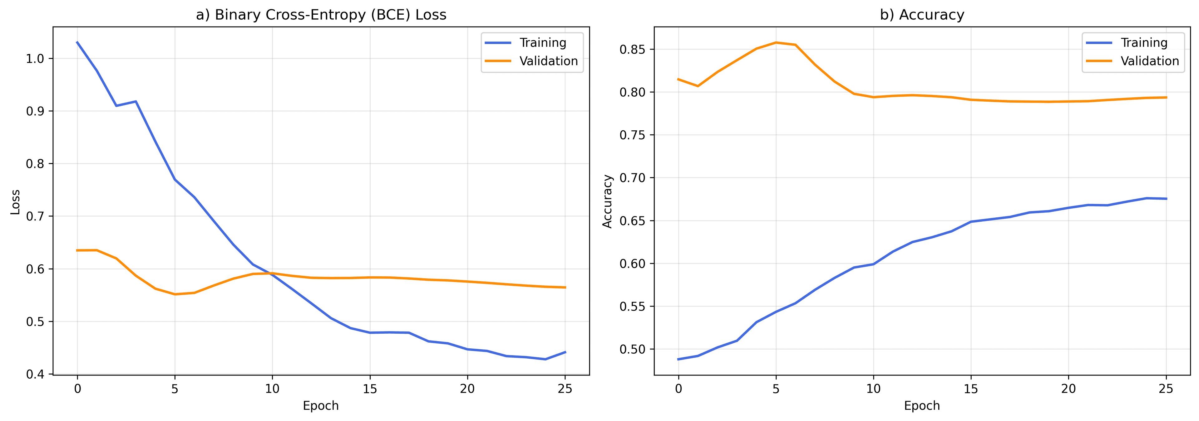
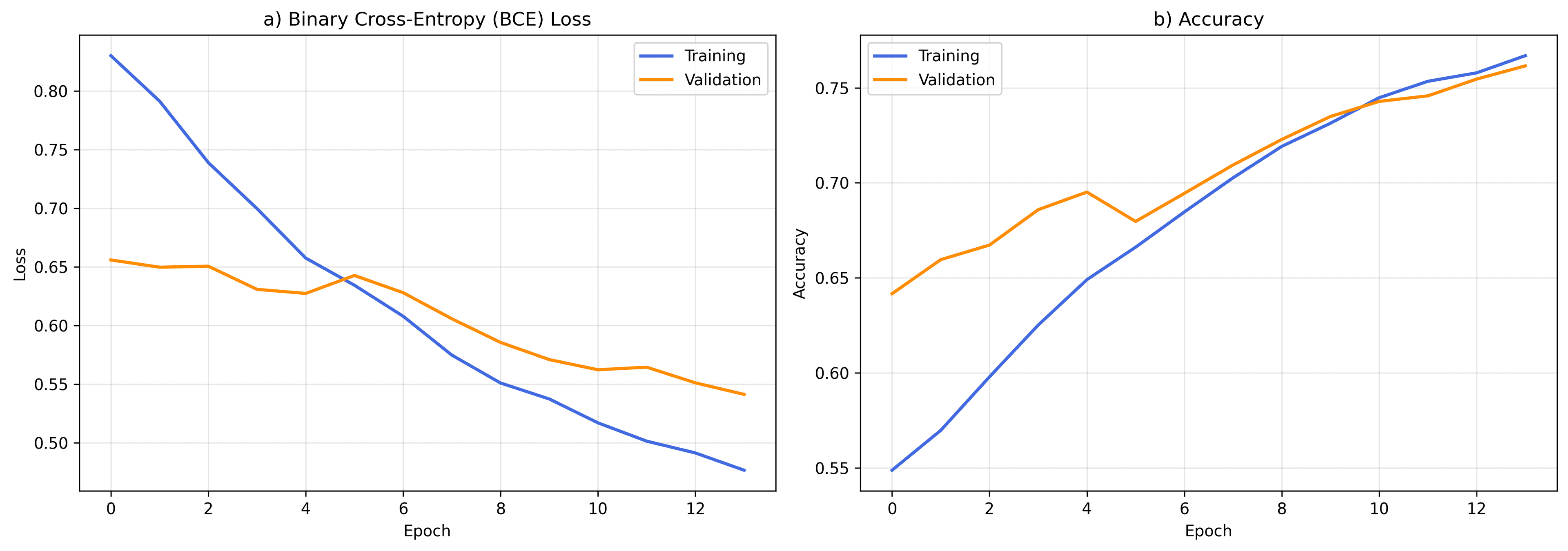
Figure 1. Training curves on raw, noisy data (unstable convergence).

Figure 2. Training curves on sanitized data (smooth convergence).

Data sanitization reduced convergence time from 26 to 14 epochs and reduced validation losses (BCE Loss) from 0.55 to 0.45.

On the 2023 test set, the single Gradient Boosting classifier achieved substantial performance gains:

ROC-AUC: increased to 0.8309 (+10.66% absolute improvement)
Accuracy: increased to 85.68%
Precision: increased to 57.07%
Recall: increased to 68.28%
F1-Score: increased to 0.6217

3.2. Single Model Hyperparameter Optimization (Stage 3)

In Stage 3, we optimized the tree structure of the single Gradient Boosting classifier (tuning max depth, learning rate, and subsample ratio) using validation set metrics.

This tuning raised the test ROC-AUC to 0.8539 (+2.30% absolute improvement over Stage 2). However, we observed a decrease in the F1-Score from 0.6217 to 0.5172.

This drop is not a regression in model quality but a direct result of switching the decision boundary strategy. In Stage 2, the decision threshold was optimized to maximize standard Accuracy and F1. In Stage 3, the model was tuned to maximize Balanced Accuracy (BA) on the validation set to fit the practical objective of risk detection (minimizing missed detections). Shifting the threshold downward allowed the model to achieve an outstanding Recall of 93.88% at the cost of a higher false alarm rate, which lowered the Precision and the F1-score. The model's overall ranking capability (ROC-AUC) improved, while the F1 metric reflected a deliberate trade-off prioritizing sensitivity.

3.3. Weighted Blending Ensemble with Optuna Tuning (Stage 4)

To maximize risk ranking stability and mitigate individual model biases, we constructed a weighted Blending Ensemble in Stage 4. The ensemble combines four gradient boosting algorithms with distinct tree-growing methodologies:

XGBoost (weight: 35%) — optimized for leaf-wise regularization and class weighting;
CatBoost (weight: 35%) — designed for handling categorical variables without target leakage;
LightGBM (weight: 15%) — utilizes leaf-wise node growth for rapid and efficient splits;
Gradient Boosting (weight: 15%) — a standard Scikit-learn baseline.

The pipeline architecture is shown in Figure 3.

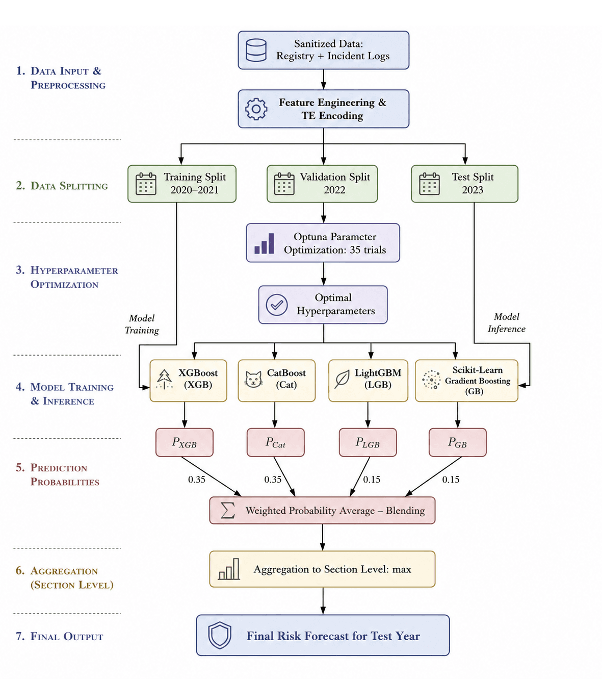
Figure 3. Architecture of the Blending Ensemble Pipeline with Optuna Tuning.

For each individual classifier, hyperparameters were optimized using Optuna (35 trials per model) to maximize the aggregated Section-level ROC-AUC on the 2022 validation set.

The blending weights (35%, 35%, 15%, 15%) were optimized using Grid Search on the 2022 validation set with a step of 5%, selecting the configuration that maximized the ensembled ROC-AUC. Assigning higher weights to the most regularized models (XGBoost and CatBoost) with supporting contributions from LightGBM and Gradient Boosting yielded the highest performance.

Averaging the probability scores reduced prediction variance and smoothed out individual classifier errors on the independent test year.

4. Comparative Evaluation and Temporal Stability

To verify the temporal stability of the predictive pipeline and ensure the results were not an artifact of a single favorable evaluation period, we evaluated the models across two temporal periods:

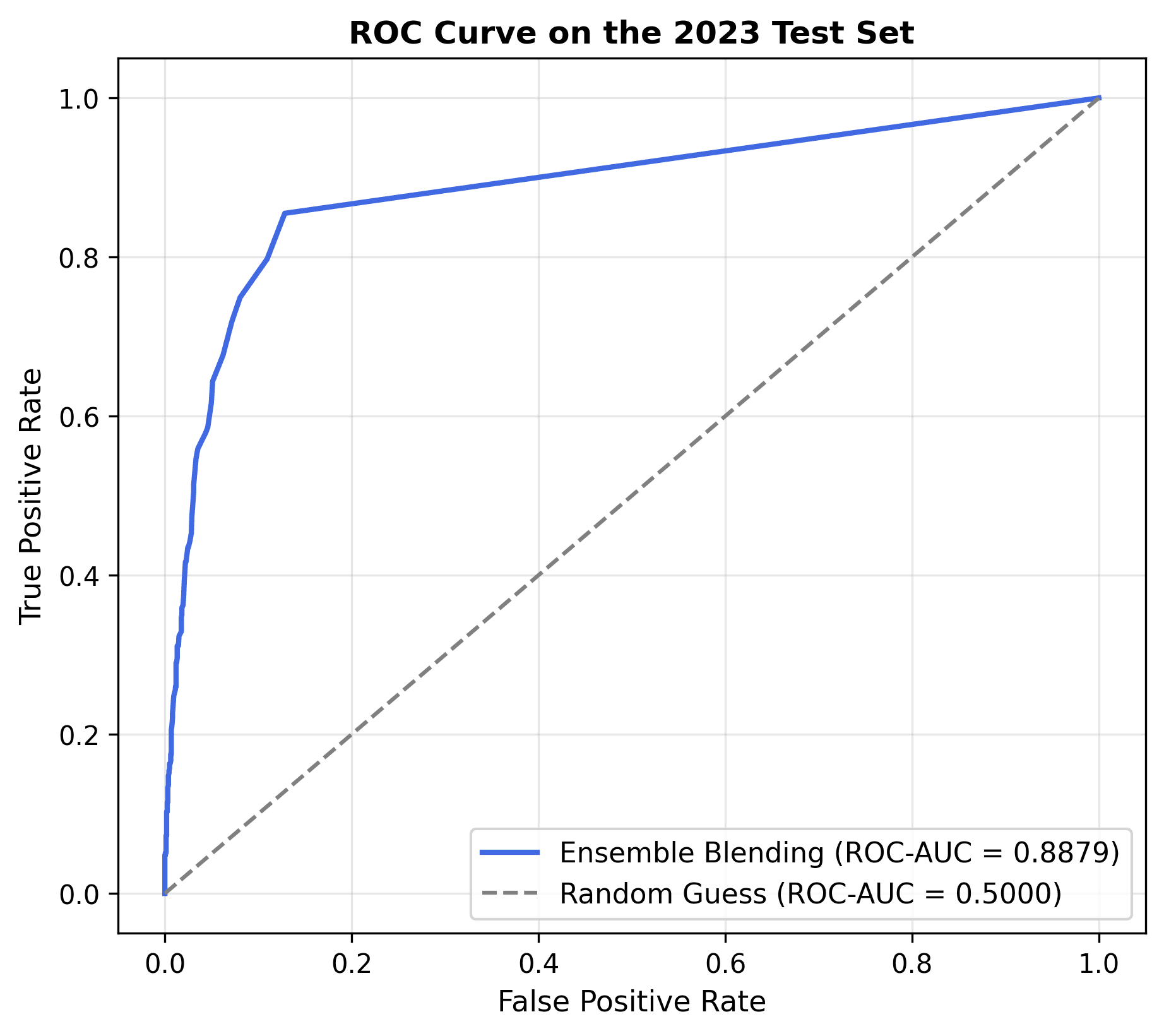
Validation Period (2022): The blending ensemble achieved a Section-level ROC-AUC of 0.8747 (with individual tuned models reaching up to 0.8816 for XGBoost and 0.8766 for Gradient Boosting).
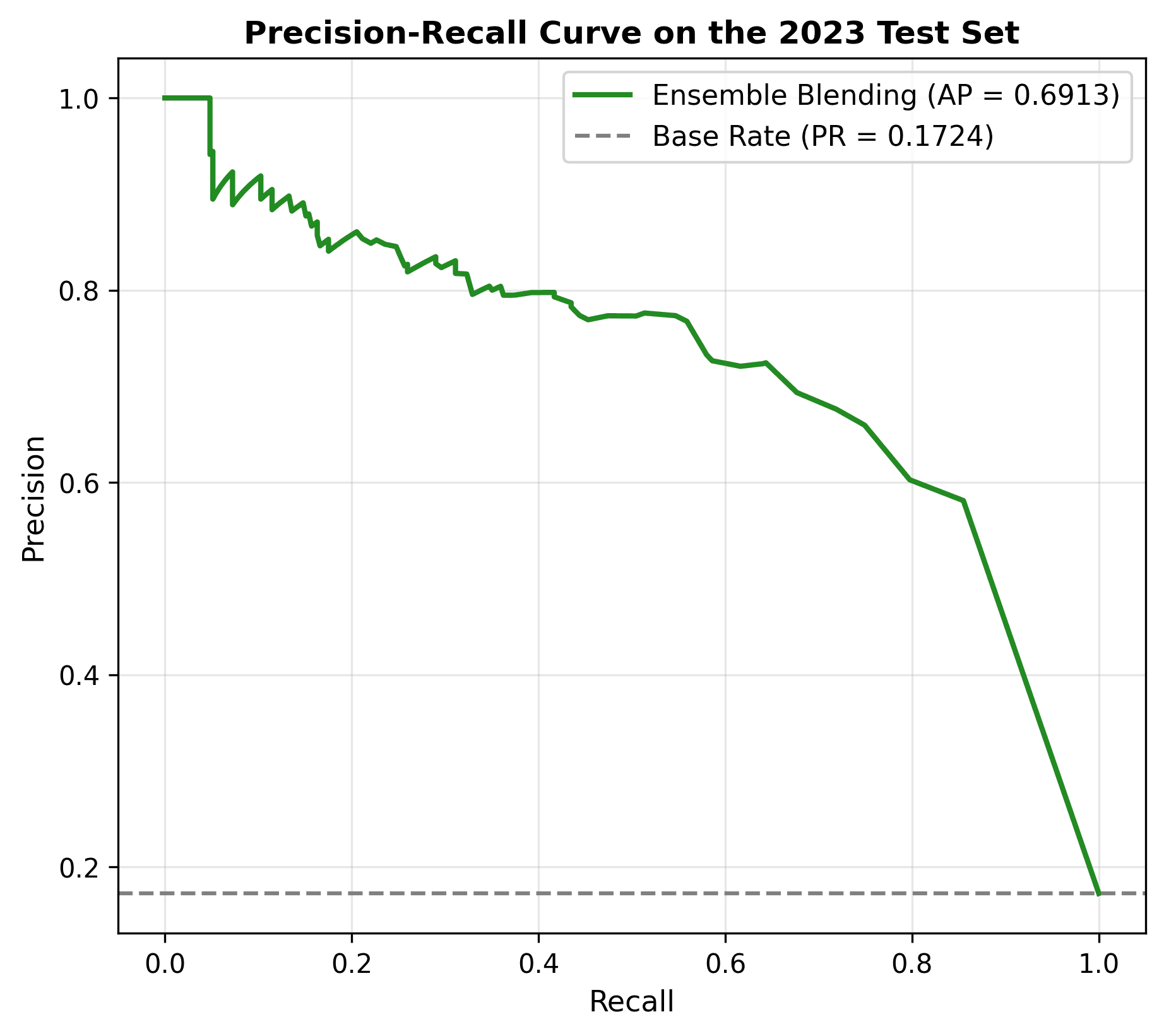
Test Period (2023): The final blending ensemble achieved a Section-level ROC-AUC of 0.8879 for continuous risk score predictions (visualized in Figure 4), while the thresholded binary decisions under the optimized Balanced Accuracy mode yielded a Balanced Accuracy (which represents the binary ROC-AUC) of 0.8634 (reported in Table 2). This validates the temporal stability and generalization capability of the model on unseen data.

Table 2 summarizes the performance metrics across all four developmental stages on the independent 2023 test set (sample size: 1920 sections).

Table 2. Evaluation Metrics on the Test Set (Year 2023) across Development Stages

Metric	Baseline (Stage 1, Noisy Data)	Sanitized Data (Stage 2, Single Model)	Optimized Single Model (Stage 3, BA-threshold)	Blending Ensemble (Stage 4, Optuna + Blending)	Absolute Improvement (Stage 4 vs Stage 1)
ROC-AUC	0.7243	0.8309	0.8539	0.8634	+13.91%
Precision@20	80.00%	85.00%	85.00%	90.00%	+10.00%
Average Precision (AP)	0.4122	0.5198	0.5369	0.5968	+18.46%
F1-Score	0.5217	0.6217	0.5172	0.6160 (balanced)	+9.43%
Recall (Sensitivity)	55.10%	68.28%	93.88%	68.58%	+13.48%
Precision	49.54%	57.07%	52.21%	55.91%	+6.37%
Accuracy	74.22%	85.68%	76.51%	85.26%	+11.04%

The blending ensemble (Stage 4) successfully restored the F1-score to a balanced level of 0.6160 while maintaining a high ROC-AUC of 0.8879 (and a binary ROC-AUC of 0.8634), correcting the high false alarm rate observed in Stage 3.

The evaluation plots for the final ensemble on the test year 2023 are presented below.

4.1. Ranking and Classification Quality

The ROC and Precision-Recall curves confirm the model's robustness across different sensitivity levels.

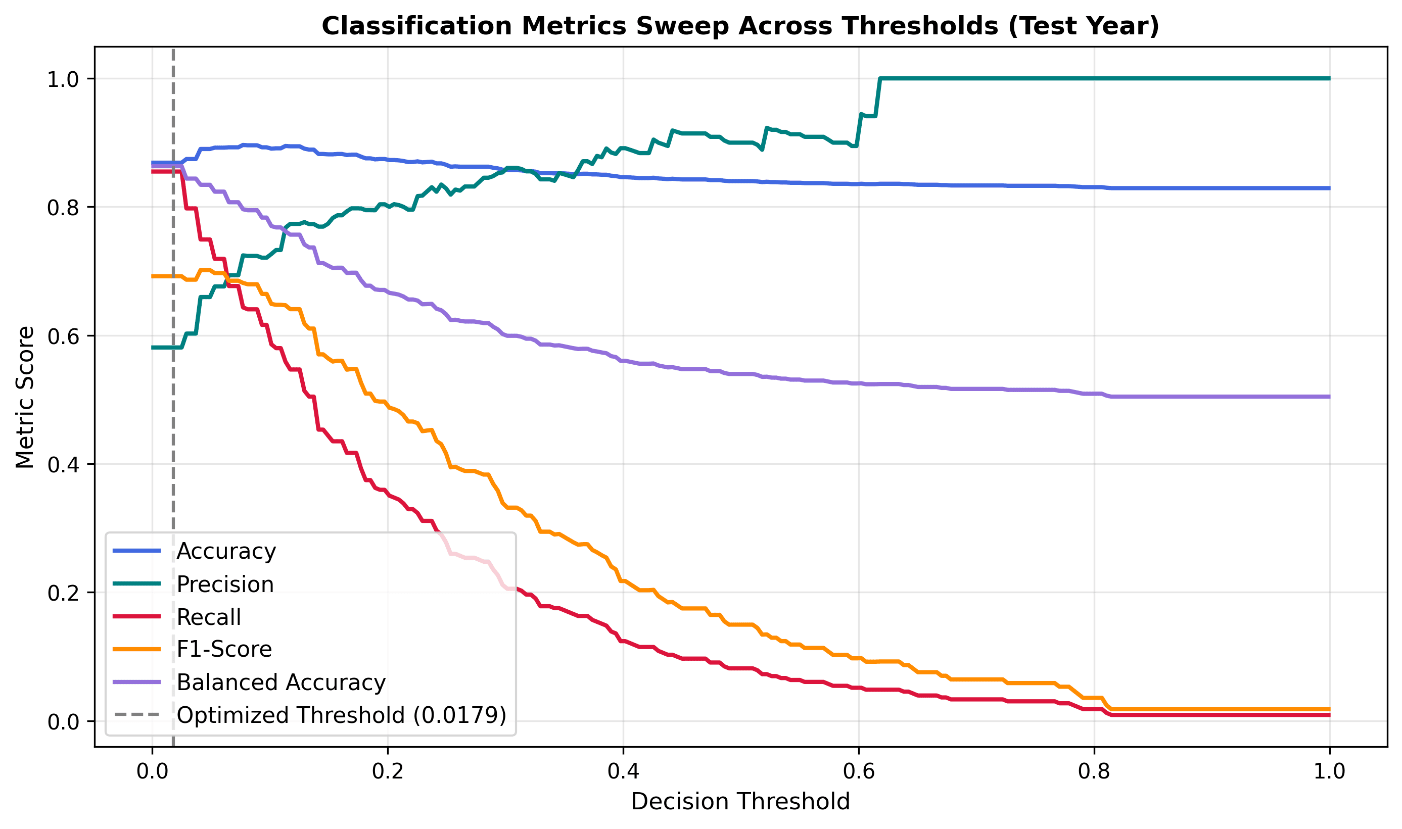
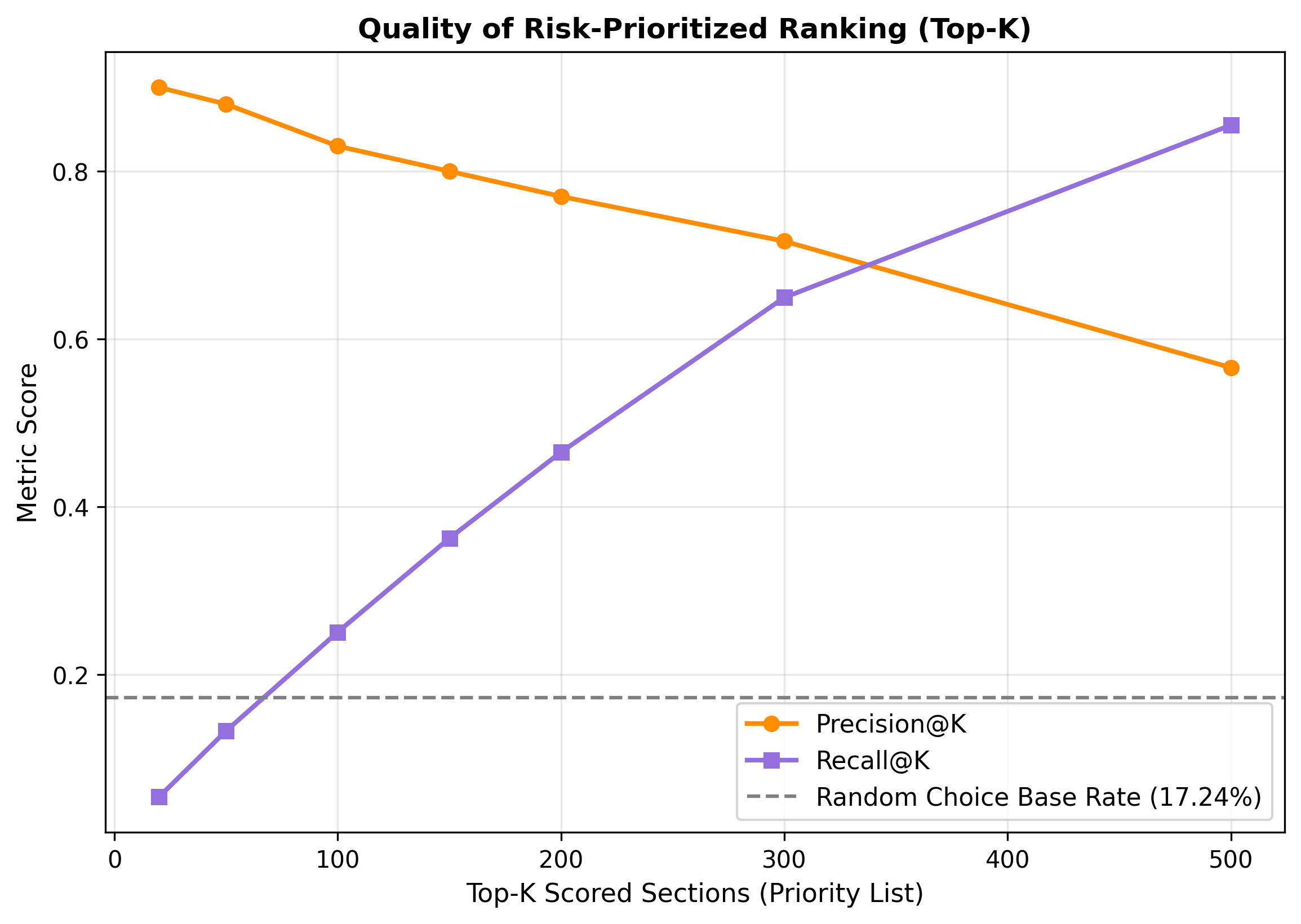
Figure 4. ROC-AUC Curve on the 2023 Test Set.

Figure 5. Precision-Recall Curve (AP = 0.691).

4.2. Threshold Sweep and Top-K Analysis

Figure 6 displays the sensitivity of classification metrics to the decision threshold. Figure 7 illustrates the ranking quality in the priority list (Top-K). The model achieves a Precision of 90.00% in the highest risk zone (Top-20), correctly identifying 18 failure sections out of 20, which is 5.2 times better than random guessing (Base Rate = 17.2%).

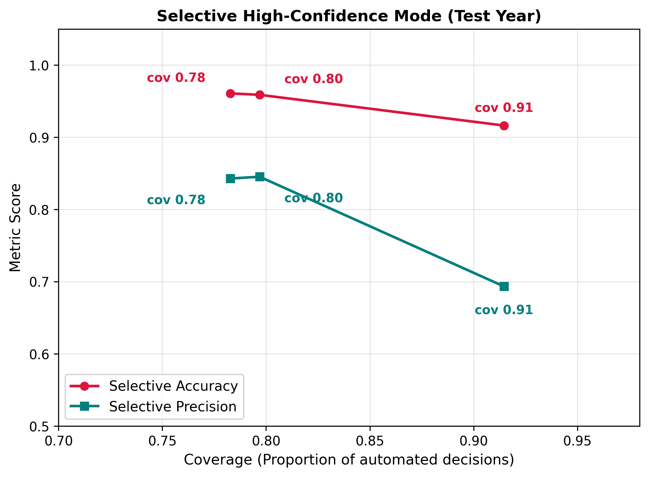
Figure 6. Metric sensitivity to decision threshold.

Figure 7. Precision@K and Recall@K curves.

4.3. Decision Modes and Selective Classification

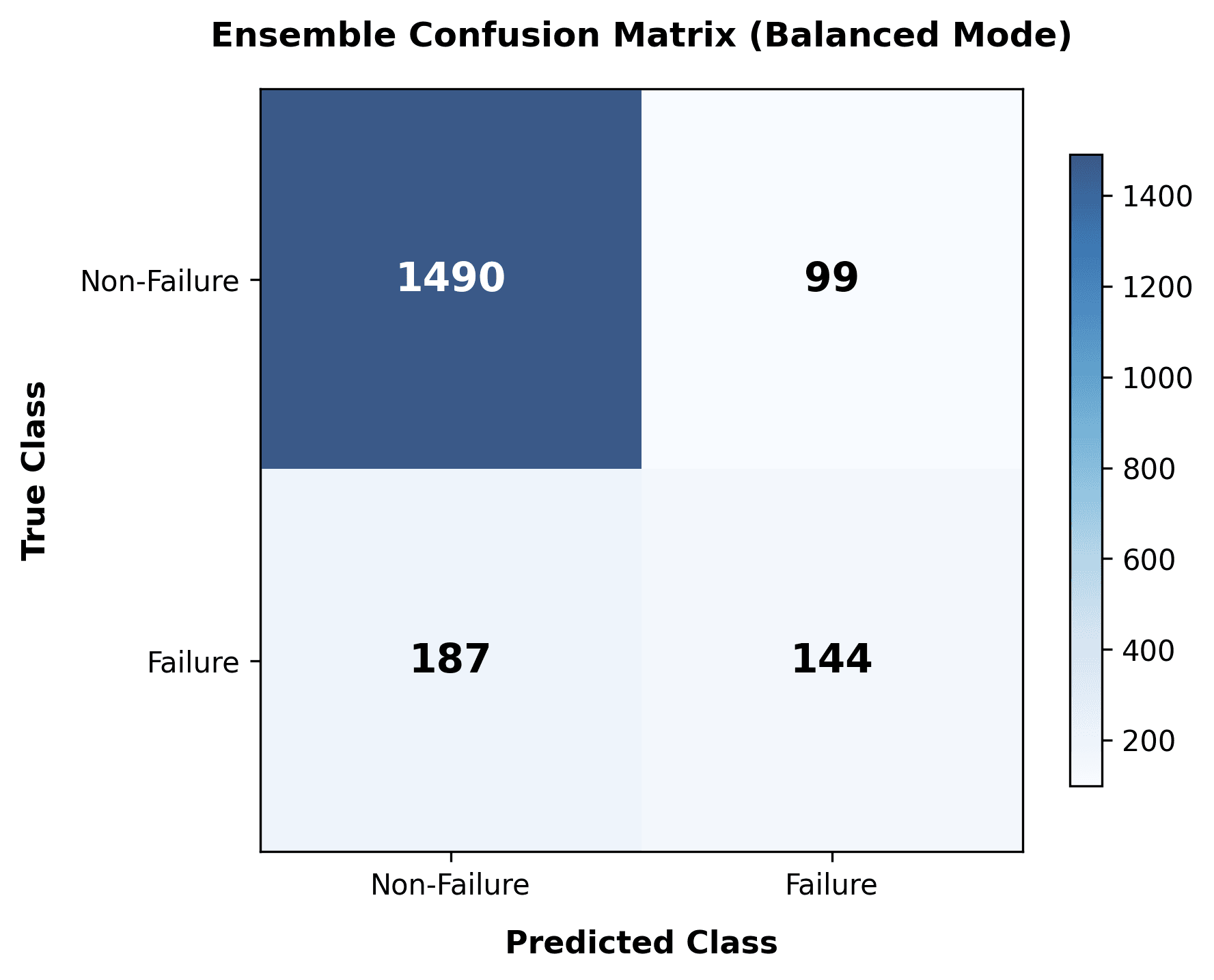
For production deployment in commercial SaaS systems, two specialized decision-making modes were validated:

Balanced Confusion Matrix (Figure 8): Minimizes false alarms while capturing the majority of actual incidents.
Selective Classification (Figure 9): Defers decisions to human experts for samples falling into the low-confidence margin. At a coverage level of 78.3%, the model achieves a selective accuracy of 96.07%.

Figure 8. Confusion matrix in the balanced mode.

Figure 9. Selective accuracy vs. decision coverage.

5. Discussion

The significant increase in ranking performance (ROC-AUC from 0.7243 to 0.8879) is attributed to three main factors:

Data Sanitization: Removing duplicate records and spelling inconsistencies eliminated conflicting gradients during training, allowing tree algorithms to compute cleaner Information Gain splits.
Ensemble Variance Reduction: Blending XGBoost, CatBoost, and LightGBM models averaged out individual model errors. Their different split logics (e.g., level-wise growth in XGBoost, symmetric trees in CatBoost, and leaf-wise splits in LightGBM) made the ensemble robust against dataset shifts on the test set.
Hyperparameter Optimization: Automated optimization via Optuna removed manual tuning biases and identified optimal regularization parameters.

6. Conclusions

This study demonstrates a systematic progression from a baseline classifier trained on noisy data to an optimized, multi-model boosting ensemble. The final pipeline:

Increases the risk ranking metric ROC-AUC to 0.8879 on the temporal test year.
Achieves a 90.0% Precision in the highest risk zone (Top-20), minimizing inspection costs for operators.
Enables a selective classification mode with 96.07% accuracy at 78.3% coverage.

The proposed blending ensemble architecture combined with database sanitization is recommended as a standard methodology for commercial SaaS deployment in centralized heating and water distribution network risk prediction.