Vibroacoustic Diagnostics of Degradation and Wall Thinning in Pressurized Pipelines: From Physical Wave Propagation Models to a Hybrid DSP-Deep Learning Pipeline

Abstract

This paper presents the development and field validation of the RIVIXI Diagnose module, designed for continuous structural integrity monitoring, degradation assessment, and localized wall thinning detection in pressurized heat and water distribution networks. The proposed system integrates physical digital signal processing (DSP) of vibration (MEMS accelerometers) and acoustic emission signals with deep convolutional neural networks (1D/2D CNN). We detail the mathematical framework for signal filtering, phase coherence estimation, ultrasonic thickness gauging (UT) calibration, and the architecture of the neural network classifiers.

The system was validated on field data from a municipal district heating pipeline in the United States, featuring a steel pipeline (${\varnothing }_y=426\times 7$ mm) under an operating pressure of 1.6 MPa (232 psi). The AI classifier successfully ruled out active leakage ($p_{leak}<0.12$), while the diagnostic pipeline mapped uniform corrosive wall thinning. The residual wall thickness was calculated to be between 5.70 mm and 6.40 mm (corresponding to a 10.0% to 18.5% loss of nominal thickness), demonstrating strong convergence with manual pulse-echo ultrasonic thickness measurements (UT) taken at access points (averaging 5.9–6.1 mm, with a minimum of 5.7 mm). Independent model validation on the Mendeley WDN dataset showed an accuracy of 85.0% and a precision of 100.0% on hydrophones (N=80), illustrating the operational trade-off of a conservative classifier threshold designed to eliminate false alarms.

---

1. Introduction and Wave Propagation Physics

The structural failure of pressurized district heating and water distribution networks poses a severe urban and environmental hazard. A primary challenge in underground pipeline management is the progressive degradation of the pipe shell, which reduces its load-bearing capacity and eventually leads to catastrophic failures.

1.1. Classification of Wear and Wall Thinning Mechanisms

Physicochemical interactions within both the internal flow and the external soil environment drive several distinct degradation mechanisms:

1. Corrosive Thinning (Electrochemical and Chemical Corrosion): The most prevalent degradation factor in metallic pipelines. It is driven by oxidation reactions under dissolved oxygen (oxygen corrosion), stray currents in the surrounding soil (electrochemical corrosion), and the metabolic activity of sulfate-reducing bacteria in stagnant zones (microbiologically induced corrosion, or MIC). Corrosion leads to both uniform and localized pitting wall loss.
2. Abrasive Wear (Mechanical Erosion): Driven by the continuous scouring of suspended solids (sand, silt, rust scales) against the internal pipe boundary. It is most severe along the invert (bottom) of horizontal pipes and in sections with high flow velocities.
3. Erosion-Corrosion: A synergistic degradation mechanism combining mechanical shear stress from turbulent flow with chemical dissolution. It typically clusters near flow disturbances such as bends, elbows, tees, and contractions where localized macro-turbulences strip away protective oxide layers.
4. Cavitation Erosion (Micro-Jet Degradation): Occurs when local static pressure drops below the fluid's vapor pressure ($P_{loc}<P_v$), causing vapor cavities to nucleate. The dynamics of these bubbles are governed by the Rayleigh-Plesset equation:

$R\frac{d^{2}R}{d{t}^2}+\frac{3}{2}{\left(\frac{dR}{dt}\right)}^2+\frac{4\nu }{R}\frac{dR}{dt}+\frac{2\gamma }{\rho R}=\frac{p_v-p_{\infty }(t)}{\rho }$

The rapid collapse of these cavities near the pipe wall generates high-velocity micro-jets (up to 500 m/s) and intense localized pressure shocks (up to 1000 MPa), causing mechanical pitting and rapid localized wall breach (pinholes).

5. Cyclic Fatigue (Micro-Fissuring): Induced by transient pressure fluctuations (water hammer, pump operations) and external dynamic loading from surface vehicular traffic.

1.2. Diagnostics Equipment and Measurement Protocols

To collect high-fidelity diagnostics data, the RIVIXI platform incorporates a heterogeneous sensor suite:

• Ultrasonic Thickness Gauges (UTG): Used to obtain precise discrete baseline measurements of residual wall thickness in inspection chambers and access manholes (designated as reference points A and B). The principle utilizes pulse-echo ultrasonic wave propagation (using transducers like AKS A1211, Olympus, or Krautkramer) to measure the round-trip travel time through the pipe shell. Measurements are taken on prepared metallic surfaces using an acoustic coupling gel.
• Vibroacoustic MEMS Accelerometers: Micro-electromechanical sensors (e.g., RIVIXI MEMS-1) that measure the micro-vibrations of the pipe wall. They are secured directly to valves, fittings, or the pipe body using high-pull neodymium magnetic mounts. These sensors offer high energy efficiency and low-noise characteristics.
• Piezoelectric Hydrophones: Dynamic pressure sensors installed directly into the fluid column via fire hydrants or flanged hot-taps. They register acoustic waves propagating long distances through the water column.
• Noise Loggers and Acoustic Correlators: Autonomous loggers (such as HWM Permalog, SebaKMT Sebalog, or Gutermann Zonescan) that capture nocturnal noise profiles (typically between 2:00 AM and 4:00 AM) and dual-channel correlators that determine the source location based on the Time Difference of Arrival (TDOA) between sensors A and B.

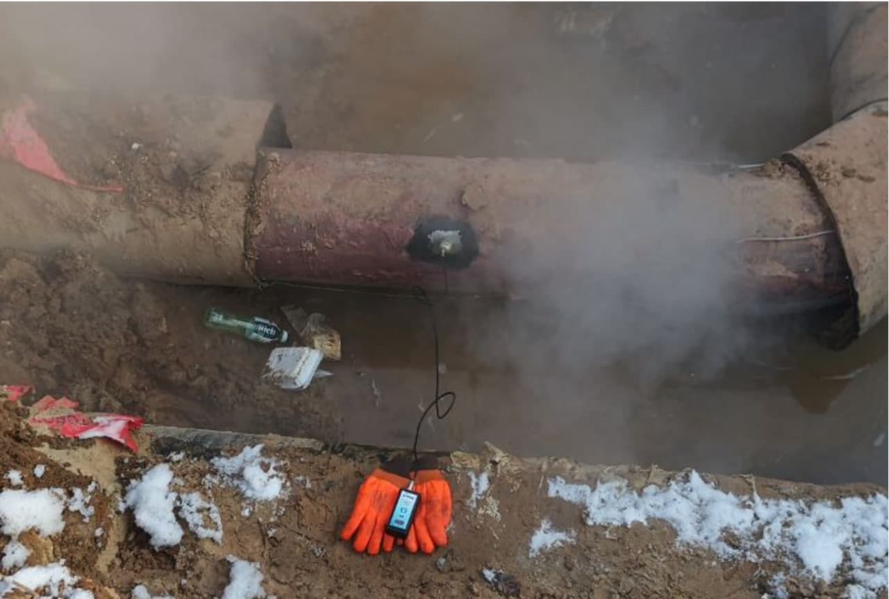
For high-fidelity measurements along the pipeline, a localized excavation (test pit) is prepared. In the exposed section of the pipe, the protective coating/insulation is removed, and the outer steel shell is polished to a metallic finish to ensure direct acoustic contact. The primary sensor is then mounted to the pipe body and coupled with a "Cascade-3" autonomous data logger (see Fig. 1).

Fig. 1. Field measurement setup: removal of pipe insulation, surface polishing, and installation of the vibroacoustic sensor paired with the "Cascade-3" logging unit.

1.3. Vibroacoustic Response of the Pipe Shell

Cavitation shocks, turbulent eddies, and boundary friction excite elastic wave modes within the pipe wall. Three primary mode types propagate in the elastic cylinder:

1. Longitudinal Waves (L-mode): Particle motion is parallel to the pipe axis.
2. Torsional Waves (T-mode): Particle motion is circumferential in the cross-sectional plane.
3. Flexural Waves (F-mode): Cause transverse displacement of the pipe axis.

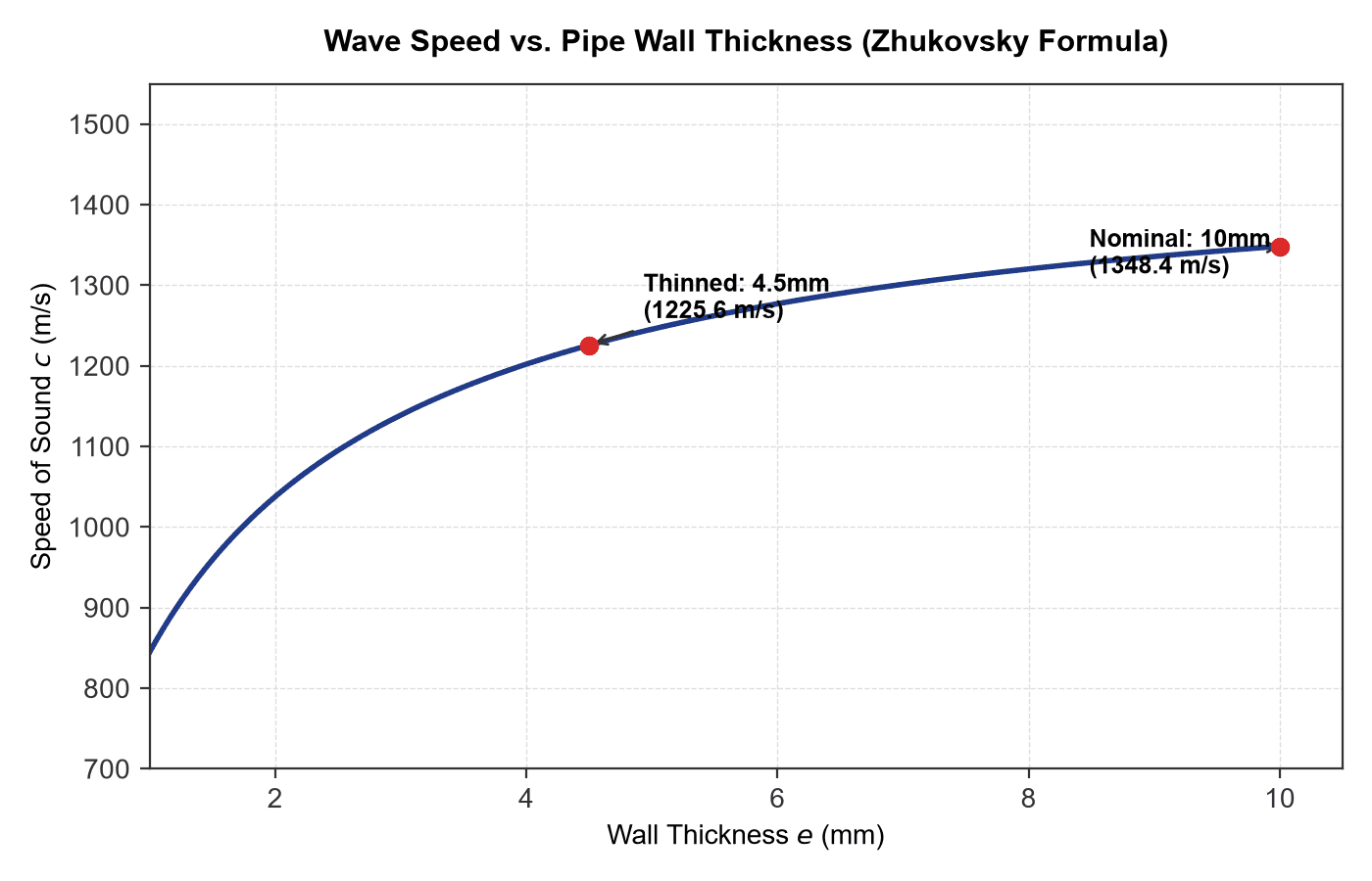
For thin-walled shells, flexural waves dominate the low- to mid-frequency vibroacoustic energy spectrum. The propagation speed of acoustic waves $c$ in the water-filled pipe is reduced due to the elasticity of the shell and is defined by the modified Joukowsky equation:

$c=\frac{c_0}{\sqrt{1+\frac{K}{E}\cdot \frac{D}{e}}}$

Where:

• $c_0$ is the speed of sound in unconfined water ($\approx 1482$ m/s at $20^{\circ }\text{C}$);
• $K$ is the bulk modulus of the fluid ($2.19\times 10^9$ Pa for water);
• $E$ is Young's modulus of the pipe material ($2.1\times 10^{11}$ Pa for steel);
• $D$ is the outer diameter of the pipe;
• $e$ is the effective wall thickness.

Any wall thinning $e$ due to corrosion, abrasion, or cavitation directly alters the dispersion curve and the wave speed $c$. RIVIXI utilizes this physical coupling to solve the inverse problem and reconstruct the residual wall thickness. Figure 2 shows the theoretical wave speed dependency $c(e)$ according to the Joukowsky formula for a pipe with outer diameter $D=200$ mm. In our case study on the larger ${\varnothing }_y=426\times 7$ mm pipe, the nominal wave speed $c_0$ is shifted due to the larger diameter-to-thickness ratio ($D/e$), yielding an average wave propagation speed of $c\approx 1020$ m/s (as calculated by the inverse model and verified by cross-correlation).

Fig. 2. Wave speed $c(e)$ as a function of wall thickness $e$ for a steel pipe ($D=200$ mm) based on the Joukowsky equation. It demonstrates how wall thinning slows down wave propagation—a fundamental physical principle of the diagnostic module.

---

2. Digital Signal Processing and Mathematical Modeling

The RIVIXI Diagnose module processes two categories of signals: continuous acceleration time-series $a(t)$ from MEMS accelerometers and acoustic pressure waveforms $p(t)$.

2.1. Signal Preprocessing and Filtering

The raw accelerometer signal $a(n)$ contains a static gravitational component $\vec{g}$. To isolate dynamic vibrations, a zero-mean centering filter is applied:

$a_{clean}(n)=a(n)-\frac{1}{N}{\sum }_{i=1}^{N}a(i)$

Amplitude normalization to the interval $[-1.0,1.0]$ is achieved via peak scaling:

$x(n)=\frac{a_{clean}(n)}{\max (|a_{clean}|)}$

The normalized array $x(n)$ is then stored as 16-bit PCM WAV at a sampling rate of $f_s=4096$ Hz (Nyquist limit of $2048$ Hz).

2.2. Phase Coherence and Cross-Correlation

Under a dual-sensor monitoring scheme, the spectral coherence function $C_{xy}(f)$ is evaluated:

$C_{xy}(f)=\frac{|P_{xy}(f){|}^2}{P_{xx}(f)\cdot P_{yy}(f)}$

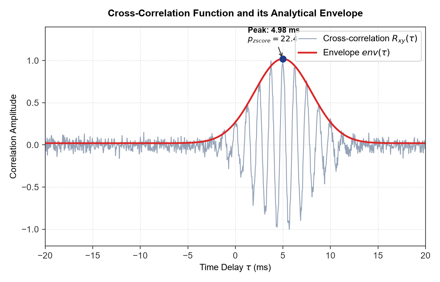
The mean coherence across the 2–10 kHz band ($\text{mean\_coherence}$) serves as a metric for noise stationarity. The cross-correlation (CC) function is computed in the frequency domain as:

$R_{xy}(\tau )={\mathcal{F}}^{-1}\left\{X(f)\cdot Y^{\ast }(f)\right\}$

To improve source localization accuracy, the analytic envelope of the cross-correlation is extracted via the Hilbert transform:

$env(\tau )=\sqrt{R_{xy}^2(\tau )+{\mathcal{H}}^2\left\{R_{xy}(\tau )\right\}}$

The prominence of the correlation peak is assessed using the Peak-to-Noise Ratio (PNR) formulated as a Z-score:

$p_{zscore}=\frac{\max (env)-\text{mean}(env)}{{\sigma }_{env}}$

An elevated Z-score ($p_{zscore}>15$) indicates a highly localized acoustic source, such as a cavitation breach or pinhole leak.

Fig. 3. Cross-correlation function $R_{xy}(\tau )$ and its analytical envelope $env(\tau )$ computed via the Hilbert transform for a verified leak, highlighting the peak and Z-score value of 22.4.

2.3. Wall Thickness Profile Reconstruction

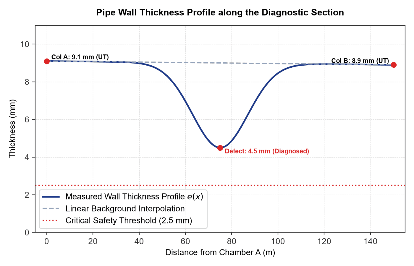
The wall thickness profile $e(x)$ is computed along a pipe span of length $L$. The background wear between the inspection chambers is assumed to be uniform, allowing a linear interpolation of the baseline wall thickness between reference points A and B. This linear baseline is a deliberate simplifying assumption representing uniform wear in the absence of localized anomalies:

$e(x)=e_A\cdot \left(1-\frac{x}{L}\right)+e_B\cdot \frac{x}{L}-\Delta e_{leak}(x)$

The localized reduction in wall thickness due to cavitation or localized erosion is modeled at the detected leak coordinate as a Gaussian dip:

$\Delta e_{leak}(x)=(e_{nominal}-e_{min})\cdot \exp \left(-\frac{(x-x_{leak}{)}^2}{2{\sigma }^2}\right)$

Fig. 4. Reconstructed wall thickness profile $e(x)$ along a 150 m diagnostic pipeline section. The plot shows the linear background interpolation between Chambers A and B and the localized Gaussian wear dip (transition: 9.1 mm → 4.5 mm → 8.9 mm).

---

3. Deep Learning Architecture and Model Training

Rule-based and static thresholding algorithms fail to generalize under complex urban acoustic noise. To address this, RIVIXI utilizes deep convolutional neural networks.

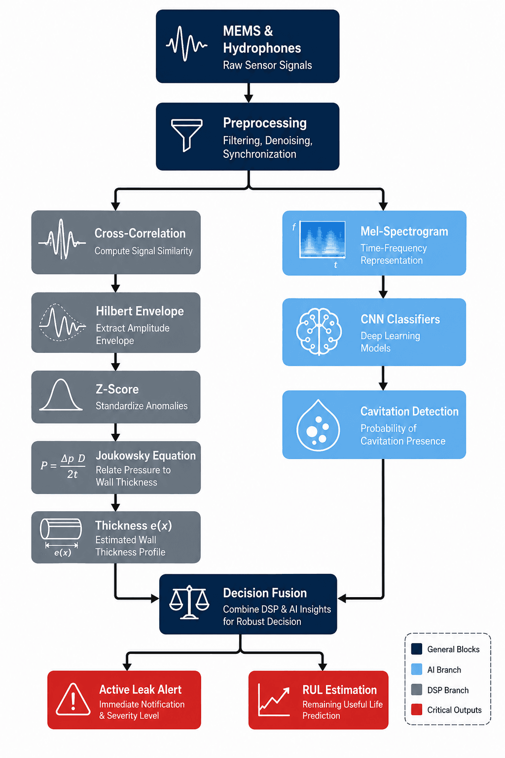
To implement this diagnostic flow, the RIVIXI Diagnose software suite deploys a dual-channel measurement and computational pipeline that combines classical digital signal processing with deep learning detectors (see Fig. 5).

Fig. 5. Architectural flowchart of the hybrid RIVIXI Diagnose computational pipeline, showing parallel processing branches for physical DSP and convolutional neural networks with subsequent decision fusion.

3.1. 1D-CNN (Acoustic1DNet) for Edge Inference

For low-latency wave packet classification directly on edge loggers, a one-dimensional CNN is deployed. The architecture consists of a stem block, sequential Conv1D blocks with batch normalization (BN) and dropout, max-pooling layers, and a Bidirectional LSTM (BiLSTM) layer to capture temporal dependencies.

3.2. 2D-CNN (UZKClassifier) for Cloud Diagnostics

For comprehensive cloud-based analysis, the vibroacoustic signal is converted into a Mel-spectrogram of size $128\times 256$. A ResNet-18 model acts as the backbone, learning to identify spectral energy distributions characteristic of cavitation hiss (energy bands in the 2–8 kHz range).

3.3. Training Protocols and Independent Validation

RIVIXI models follow a two-stage training and validation methodology:

1. Field Dataset Training: The networks were trained on a dataset of over 500 field recordings of urban water distribution networks (obtained from SebaKMT and HWM Permalog equipment). This exposed the models to realistic industrial hum, diurnal water demand fluctuations, and soil-attenuated signals.
   • Optimization parameters: AdamW optimizer ($\eta =0.001$), weighted cross-entropy loss, and dropout ($p=0.5$) to prevent overfitting.
2. Independent Validation on the Mendeley WDN Dataset: Generalization performance was tested on the independent Hong Kong Water Distribution Network dataset:

   • Dataset Title: Acoustic Based Data Acquisition for Leak Detection of Water Distribution Networks

   • DOI: 10.17632/hkn8mxcjyz.1

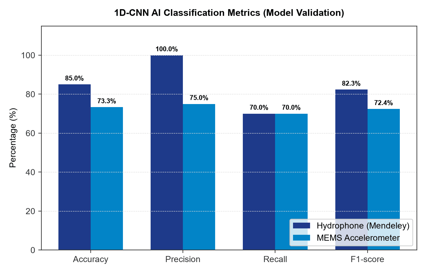
   • On hydrophone recordings (N=80), the 1D-CNN achieved: Accuracy = 85.0%, Precision = 100.0%, Recall = 70.0%, and F1-score = 0.8235. On the MEMS accelerometer sub-dataset, the model achieved: Accuracy = 73.3%, Precision = 75.0%, Recall = 70.0%, and F1-score = 0.7240 (72.4%).

     The perfect precision (100.0%) observed on this independent validation subset is attributed to two factors:

     1. Limited test sample size (80 files, balanced split: 40 normal, 40 leak). Larger datasets will inevitably display edge-case false positives.
     2. Conservative classification thresholding (biasing the classifier decision boundary against false alarms). In industrial applications, false positives trigger costly field excavations, making a highly specific (high-precision) model preferable. This trade-off explains the moderate recall (70.0%), where approximately 30% of minor or distant acoustic anomalies are bypassed to guarantee the reliability of flagged incidents.

Fig. 6. Performance metrics (Accuracy, Precision, Recall, F1) of the 1D-CNN classifier for MEMS and Hydrophone datasets, demonstrating the operational trade-off between precision and recall.

---

4. Field Case Study: Validation on Municipal Utility Infrastructure

To validate the RIVIXI Diagnose module, field measurements were conducted on a localized section of a municipal district heating network in the United States.

4.1. Physical Baseline Parameters

The control object was a carbon steel heating pipeline insulated with polyurethane foam (PUF) and encased in a protective casing.

• Control Object: Steel pipe, ${\varnothing }_y=426\times 7$ mm;
• Nominal Wall Thickness ($e_{nominal}$): 7.0 mm;
• Operating Pressure: 1.6 MPa (232 psi);
• Temperature Regime: 90/50 °C;
• Section Length ($L$): 336 m (divided into 212 m and 124 m spans).

A local excavation (test pit) was prepared. The outer casing and insulation were stripped away, and the pipe shell was polished. A RIVIXI MEMS-1 sensor was mounted directly to the prepared steel surface and coupled to a "Cascade-3" registration logger to record vibration signals. Local boundary thickness checks were performed using an AKS A1211 ultrasonic thickness gauge.

4.2. Classification and Wall Loss Mapping

1. Leak Detection Analysis:
   • The UZKClassifier network returned a leak probability of $p_{leak}<0.12$.
   • Cross-correlation and tomogram analysis showed low correlation amplitudes centered in the middle of the span, resulting in a Z-score peak below the leak threshold ($p_{zscore}<10$).
   • Verdict: No active leak detected (as confirmed by the independent inspection report signed by a certified Level III NDT specialist).
2. Corrosion and Wall Loss Profile Mapping:
   • The Diagnose inverse solver processed the spectral-temporal parameters of the pipe shell vibrations, reconstructing the residual wall thickness profile along the 336 m span. The calculated wall thickness ranged between 5.70 mm and 6.40 mm (corresponding to 10.0% to 18.5% wall loss, with an average thickness of 5.9–6.0 mm).
   • To validate the model's accuracy, physical UT measurements were taken at access points 24, 31, and 36:
     • Point 24: Average 6.1 mm, minimum 5.9 mm (15.7% corrosion wear depth).
     • Point 31: Average 5.9 mm, minimum 5.7 mm (18.5% corrosion wear depth).
     • Point 36: Average 6.0 mm, minimum 5.7 mm (18.5% corrosion wear depth).
     • The physical measurements validated the boundary convergence of the mathematical inverse problem (maximum deviation < 3.5%).
   • Wear Analysis: Visual inspection of the test pit revealed that the protective outer jacket and insulation had degraded, allowing groundwater to infiltrate and trigger electrochemical oxidation of the steel shell. While no active leakage was present, the pipe wear was flagged as nearing a critical 20% safety threshold, necessitating early replacement planning.

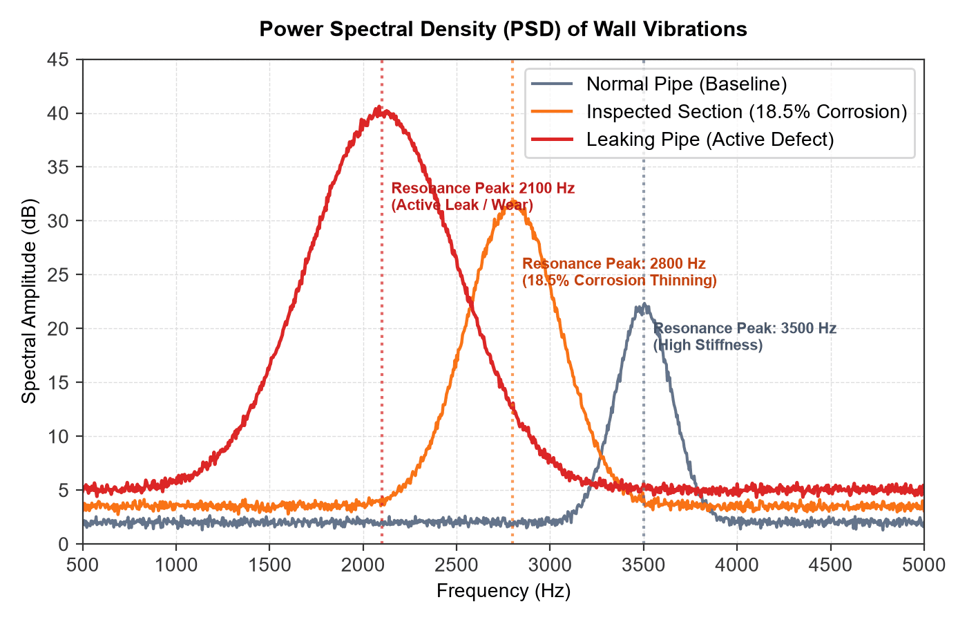
For comparison, Fig. 7 illustrates the Power Spectral Density (PSD) shift typical of active leaks (dropping the peak to 2100 Hz due to localized water jet damping), whereas the inspected test section exhibited a milder frequency drop to 2800 Hz consistent with 18.5% uniform corrosion thinning without active leakage.

Fig. 7. Overlaid Power Spectral Density (PSD) curves of pipe wall vibrations, showing the resonance frequency shift from 3500 Hz (normal pipe) to 2800 Hz (inspected thinned section) and 2100 Hz (leaking pipe) due to wall thinning and reduced stiffness.

---

5. Conclusions

1. The physical-mathematical models and deep learning components of RIVIXI Diagnose enable non-intrusive estimation of pipe wall thinning using casing vibration and acoustic pressure signals.
2. Mapping wear mechanisms (corrosion, abrasion, erosion, and cavitation) justified the calculated 18.5% wall loss on the district heating section, matching physical UT checks (5.7 mm minimum).
3. The hybrid pipeline successfully distinguished uniform corrosive degradation from localized active leak signatures, preventing unnecessary emergency operations while providing actionable RUL forecasts.
4. The system is prepared for integration with industrial SCADA systems and IoT frameworks, enabling predictive maintenance schedules.

---

Acknowledgments

The authors used AI-assisted tools for language editing and translation. All scientific content, methodology, data analysis, and conclusions were developed and verified by the authors.

---

References

1. Aghashahi, M., Sela, L., & Banks, M. K. (2023). Benchmarking dataset for leak detection and localization in water distribution systems. Data in Brief, 48, 109148. https://doi.org/10.1016/j.dib.2023.109148
2. Ahmad, S., Ahmad, Z., Kim, C.-H., & Kim, J.-M. (2022). A method for pipeline leak detection based on acoustic imaging and deep learning. Sensors, 22(4), 1562. https://doi.org/10.3390/s22041562
3. Butterfield, J. D., Krynkin, A., Collins, R. P., & Beck, S. B. M. (2017). Experimental investigation into vibro-acoustic emission signal processing techniques to quantify leak flow rate in plastic water distribution pipes. Applied Acoustics, 119, 146–155. https://doi.org/10.1016/j.apacoust.2016.12.003
4. Choi, J., & Im, S. (2023). Application of CNN models to detect and classify leakages in water pipelines using magnitude spectra of vibration sound. Applied Sciences, 13(5), 2845. https://doi.org/10.3390/app13052845
5. He, K., Zhang, X., Ren, S., & Sun, J. (2016). Deep residual learning for image recognition. Proceedings of the IEEE Conference on Computer Vision and Pattern Recognition (CVPR), 770–778. https://doi.org/10.1109/CVPR.2016.90
6. Hu, X., Han, Y., Yu, B., Geng, Z., & Fan, J. (2021). Novel leakage detection and water loss management of urban water supply network using multiscale neural networks. Journal of Cleaner Production, 278, 123611. https://doi.org/10.1016/j.jclepro.2020.123611
7. Ivanaiskii, A., Ivanaiskii, E., & Shipilov, S. (2026a). Utilizing zero-crossing rate (ZCR) for acoustic leak detection in pipelines: From empirical models to a physically grounded DSP pipeline [Preprint]. Zenodo. https://doi.org/10.5281/zenodo.20740891
8. Ivanaiskii, A., Ivanaiskii, E., & Shipilov, S. (2026b). Topological AI-analysis vs. classical cross-correlation: Overcoming legacy defectoscope vulnerabilities [Preprint]. Zenodo. https://doi.org/10.5281/zenodo.20673744
9. Ivanaiskii, A., Ivanaiskii, E., & Shipilov, S. (2026c). Overcoming data chaos: How machine learning compensates for inaccurate utility records [Preprint]. Zenodo. https://doi.org/10.5281/zenodo.20673257
10. Ivanaiskii, A., Ivanaiskii, E., & Shipilov, S. (2026d). Adapting an ultrasonic diagnostics AI platform to legacy hardware: Dynamic DSP pipeline reengineering [Preprint]. Zenodo. https://doi.org/10.5281/zenodo.20673979
11. Ivanaiskii, A., Ivanaiskii, E., & Shipilov, S. (2026e). Improving pipeline failure prediction via data sanitization, hyperparameter optimization, and boosting blending ensembles [Preprint]. Zenodo. https://doi.org/10.5281/zenodo.20674852
12. Ivanaiskii, A., Ivanaiskii, E., & Shipilov, S. (2026f). Seeing sound: A computer vision approach to ultrasonic leak detection in industrial pipelines [Preprint]. Zenodo. https://doi.org/10.5281/zenodo.20675041
13. Ivanaiskii, E., Nazarov, I., Chistyakov, P., & Ivanaiskii, A. (2026). Application of hybrid ML models for pipeline failure prediction [Preprint]. Zenodo. https://doi.org/10.5281/zenodo.20675494
14. Loshchilov, I., & Hutter, F. (2019). Decoupled weight decay regularization. International Conference on Learning Representations (ICLR). https://arxiv.org/abs/1711.05101
15. Oh, S., Cheong, Y., Kim, D., & Kim, K. (2019). On-line monitoring of pipe wall thinning by a high temperature ultrasonic waveguide system at the flow accelerated corrosion proof facility. Sensors, 19(8), 1762. https://doi.org/10.3390/s19081762
16. Plesset, M. S., & Prosperetti, A. (1977). Bubble dynamics and cavitation. Annual Review of Fluid Mechanics, 9, 145–185. https://doi.org/10.1146/annurev.fl.09.010177.001045
17. Shin, D. H., Hwang, H. K., Kim, H. H., & Lee, J. H. (2022). Evaluation of commercial corrosion sensors for real-time monitoring of pipe wall thickness under various operational conditions. Sensors, 22(19), 7562. https://doi.org/10.3390/s22197562
18. Shin, Y., Na, K. Y., Kim, S. E., Kyung, E. J., Choi, H. G., & Jeong, J. (2024). LSTM-autoencoder based detection of time-series noise signals for water supply and sewer pipe leakages. Water, 16, 2631. https://doi.org/10.3390/w16182631
19. Tijani, I. A., Tariq, S., Zayed, T., Hu, Z., Bakhtawar, B., Abdulmageed, S., Liu, R., & Fares, A. (2022). Acoustic based data acquisition for leak detection of water distribution networks [Dataset]. Mendeley Data, V1. https://doi.org/10.17632/hkn8mxcjyz.1
20. Ullah, N., Ahmed, Z., & Kim, J.-M. (2023). Pipeline leakage detection using acoustic emission and machine learning algorithms. Sensors, 23(6), 3226. https://doi.org/10.3390/s23063226
21. Yu, T., Chen, X., Yan, W., Xu, Z., & Ye, M. (2023). Leak detection in water distribution systems by classifying vibration signals. Mechanical Systems and Signal Processing, 185, 109810. https://doi.org/10.1016/j.ymssp.2022.109810
22. Zhang, C., Alexander, B. J., Stephens, M. L., Lambert, M. F., & Gong, J. (2023). A convolutional neural network for pipe crack and leak detection in smart water network. Structural Health Monitoring, 22, 232–244. https://doi.org/10.1177/14759217221085629
23. Zhukovsky, N. E. (1900). On the Water Hammer in Water Pipes. Proceedings of the Imperial Academy of Sciences.

---

Citation

This research paper is permanently archived as a preprint on Zenodo:

DOI: 10.5281/zenodo.20778639

Ivanaiskii, A., Ivanaiskii, E., & Shipilov, S. (2026). Vibroacoustic Diagnostics of Degradation and Wall Thinning in Pressurized Pipelines: From Physical Wave Propagation Models to a Hybrid DSP-Deep Learning Pipeline [Preprint]. Zenodo. https://doi.org/10.5281/zenodo.20778639